Feature Extraction by Sequence-to-sequence Autoencoder
Autoencoder
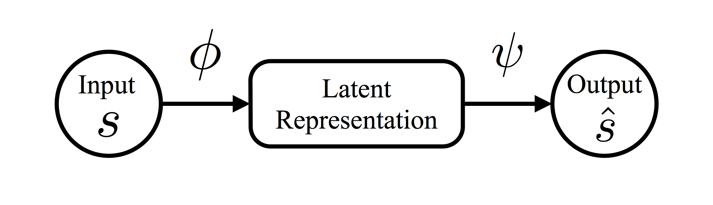
Autoencoder is a type of artificial neural networks often used for dimension reduction and feature extraction. It consists of two components, an encoder \(\phi\) and a decoder \(\psi\). The encoder \(\phi\) takes the input \(\mathbf{s}\) and transforms it into a low-dimensional vector. The decoder \(\psi\) takes the low-dimensional vector and reconstructs the input. If the reconstructed input from the autoencoder resembles the original input, the low-dimensional vector can be treated as a latent representation of the input.
 To obtain an autoencoder for a set of data, one often specifies the encoder and the decoder as a family of functions, \(\phi_{\boldsymbol \eta}\) and \(\psi_{\boldsymbol \xi}\), respectively, where \(\boldsymbol \eta\) and \(\boldsymbol \xi\) are parameters to be estimated from data. Let \(\{\boldsymbol s_1, \ldots, \boldsymbol s_n\}\) be a set of \(n\) data points and \(\hat{\boldsymbol s}_i = \psi_{\boldsymbol \xi}(\phi_{\boldsymbol \eta}(\boldsymbol s))\). Then \(\boldsymbol \eta\) and \(\boldsymbol \xi\) are estimated by minimizing \[
\begin{equation}\label{eq:obj}
F(\boldsymbol \eta, \boldsymbol \xi) = \sum_{i=1}^n L(\boldsymbol s_i, \hat{\boldsymbol s}_i),
\end{equation}
\] where \(L\) is a function measuring the difference between the reconstructed data \(\hat{\boldsymbol s}_i\) and the original data \(\boldsymbol s_i\). Once the estimated parameters \(\hat{\boldsymbol \eta}\) and \(\hat{\boldsymbol \xi}\) are obtained, the latent representation or the features of \(\boldsymbol s_i\) can be computed by \(\boldsymbol \theta_i = \phi_{\hat {\boldsymbol \eta}}(\boldsymbol s_i)\).
To obtain an autoencoder for a set of data, one often specifies the encoder and the decoder as a family of functions, \(\phi_{\boldsymbol \eta}\) and \(\psi_{\boldsymbol \xi}\), respectively, where \(\boldsymbol \eta\) and \(\boldsymbol \xi\) are parameters to be estimated from data. Let \(\{\boldsymbol s_1, \ldots, \boldsymbol s_n\}\) be a set of \(n\) data points and \(\hat{\boldsymbol s}_i = \psi_{\boldsymbol \xi}(\phi_{\boldsymbol \eta}(\boldsymbol s))\). Then \(\boldsymbol \eta\) and \(\boldsymbol \xi\) are estimated by minimizing \[
\begin{equation}\label{eq:obj}
F(\boldsymbol \eta, \boldsymbol \xi) = \sum_{i=1}^n L(\boldsymbol s_i, \hat{\boldsymbol s}_i),
\end{equation}
\] where \(L\) is a function measuring the difference between the reconstructed data \(\hat{\boldsymbol s}_i\) and the original data \(\boldsymbol s_i\). Once the estimated parameters \(\hat{\boldsymbol \eta}\) and \(\hat{\boldsymbol \xi}\) are obtained, the latent representation or the features of \(\boldsymbol s_i\) can be computed by \(\boldsymbol \theta_i = \phi_{\hat {\boldsymbol \eta}}(\boldsymbol s_i)\).
Sequence-to-Sequence Autoencoder
Process data consists of action sequences. To extract features from process data by autoencoders, we need to construct an autoencoder that takes an action sequence and produce a reconstructed action sequence. In short, we need a sequence-to-sequence autoencoder.
Encoder
Suppose that there are \(N\) possible actions. Given an action sequence, our encoder first associates each of the \(N\) unique actions with a \(K\)-dimensional numeric vector, called the embedding of the action. With this operation, an action sequence of length \(T\) is transformed into a sequence of T \(K\)-dimensional vectors. This sequence of vectors is then fed to an recurrent neural network (RNN), whose last input, denoted by \(\boldsymbol{\theta}\), is used as the output of the encoder which summarizes the information in the sequence. The parameters of the encoder are the action embeddings and the parameters in the RNN.
Decoder
The decoder of the sequence-to-sequence autoencoder utilize another RNN to reconstruct the action sequence from \(\boldsymbol{\theta}\). The decoder first replicates \(\boldsymbol{\theta}\) \(T\) times and feeds it to the decoder RNN. The same \(\boldsymbol{\theta}\) is used as the input of the decoder RNN at each time step. Then, the output vector at each time step of the decoder RNN is a summary of the action taken in that step. Let \(\mathbf{y}_t\) denote the output of the decoder RNN at time step \(t\). A multinomial logistic model is used to characterize the distribution of the action. Specifically, the probability that action \(j\) is taken at time \(t\) is proportional to \(\exp(b_j + \boldsymbol y_t^\top \boldsymbol \beta_j)\). Note that the parameters \(b_j\) and \(\boldsymbol \beta_j\) do not depend on \(t\). The probability vectors at \(T\) time steps are the output the decoder. The decoder essentially specifies a probabilistic model of action sequences. The parameters of the decoder are the parameters in the decoder RNN and the coefficients in the multinomial logistic model.
Loss
We use cross entropy to measure the discrepancy between the original and the reconstructed action sequences:
\[\begin{equation} L(\mathbf{S}, \hat{\mathbf{S}}) = -\frac{1}{T}\sum_{t=1}^T \sum_{j=1}^N S_{tj} \log(\hat{S}_{tj}), \end{equation}\]
where \(S_{tj}\) is an indicator of whether the \(t\)th action in the action sequence is action \(a_j\) and \(\hat{S}_{tj}\) is probability that the action at \(t\)th step is \(a_j\). Note that only one of \(S_{t1}, \ldots, S_{tN}\) is non-zero. The loss function is smaller if the distribution specified by \((\hat{S}_{t1}, \ldots, \hat{S}_{tN})\) is more concentrated in the action that is actually taken. Given the latent representation \(\boldsymbol \theta\), the loss function is essentially the negative log-likelihood of the input action sequence under the model specified by the decoder. With this loss function, we can estimate the parameters in the sequence-to-sequence autoencoder by minimizing the objective function \(L\).
Feature Extraction Procedure
The procedure to extract features from process data by sequence-to-sequence autoencoder can be summarized as follows.
Construct the sequence-to-sequence autoencoder by finding \(\hat{\boldsymbol \eta}\) and \(\hat{\boldsymbol \xi}\) as the minimizer of with \(L\) defined in .
Compute \(\tilde{\boldsymbol{\theta}}_i = \phi_{\hat{\boldsymbol{\eta}}}(\mathbf{S}_i)\), for \(i = 1, \ldots, n\). Each column of \(\tilde{\Theta} = (\tilde{\theta}_1, \ldots, \tilde{\theta}_n)^\top\) is a raw feature for the process data.
Obtain \(K\) principal features by performing principal analysis on the raw features \(\tilde{\Theta}\).